Transmissivity measures how readily an aquifer passes water; a district reads it from the drawdown slope of a constant-rate, recovery or step test. Transmissivity belongs to the aquifer and well loss to the well, so tracking both shows which changed.
A district with pumping tests on file already holds what it needs. Below are the arithmetic for each, one example well worked through all of them, and the reason specific capacity alone understates transmissivity on any well with well loss.
What is transmissivity, and what units does a district use?
Transmissivity (T) is the rate at which water moves through a strip of aquifer one foot wide, across its full saturated thickness, under a hydraulic gradient of one foot per foot. It equals hydraulic conductivity times saturated thickness, which makes it a property of the aquifer around the well, not of the well.
District practice gives T in gallons per day per foot (gpd/ft); divide by 7.48, the gallons in a cubic foot, for ft²/day. Storativity (S) is the water an aquifer releases per unit area per foot of head decline. A test on the pumping well alone gives T but not a usable S; that takes an observation well.
How do you calculate transmissivity from a constant-rate test?
Use the Cooper–Jacob straight-line method (Cooper and Jacob, 1946). Plot drawdown on the arithmetic axis against time since pumping began on the log axis. Once u = r²S ÷ (4Tt) is small, which the U.S. Geological Survey’s treatment puts at generally less than 0.01 (Ferris and others, 1962), the points fall on a straight line. Its slope gives T:
T = 264 Q ÷ Δs
T in gpd/ft; Q, the constant pumping rate, in gpm; Δs, the rise in drawdown over one log cycle of time (10 to 100 minutes, or 100 to 1,000), in ft. The 264 comes from the Cooper–Jacob slope, Δs = 2.303 Q ÷ (4πT) in consistent units. Converting gpm to gallons per day multiplies Q by 1,440, and 2.303 × 1,440 ÷ (4π) = 263.9, rounded to 264.
At the pumping well, r is only the well’s radius, so u becomes small quickly; the first minutes there are spoiled instead by casing storage, water drawn from the casing itself. Fit the line after that and before a boundary or leakage bends it. Well loss does not change the slope: at a constant rate it adds the same feet to every reading. So the slope still gives T at the pumping well, while the line’s position does not give S.
Single-well results are usable, with one caveat. In 628 simulated single-well tests, Cooper–Jacob estimates for confined aquifers were affected minimally by partial penetration, vertical anisotropy or the analyst; for unconfined aquifers they averaged twice the known values (Halford and others, 2006). Late-time data improved the unconfined estimates where T exceeded 250 m²/day, about 20,100 gpd/ft.
Can you get transmissivity from recovery data?
Yes, and often more cleanly. Theis (1935) showed that after a pump stops, the residual drawdown behaves as if the well had kept pumping and a recharge well of the same rate had started at the same point at the moment of shutdown. Subtract the two Cooper–Jacob lines and S and the radius cancel:
T = 264 Q ÷ Δs′
Q is the rate pumped before shutdown, in gpm. Δs′ is the change in residual drawdown, in ft, over one log cycle of t ÷ t′, where t is time since pumping began and t′ is time since it stopped. Plot residual drawdown against log(t ÷ t′). The small-u condition still applies, now with t′.
Once the pump stops, only the water refilling the casing flows through the screen, so the well-loss term drops out. Water draining back down the pump column can disturb the first readings; read the slope from the later, straight part of the plot.
How do you get transmissivity from a step-drawdown test?
A step test pumps the well at several rates in steps of equal length. Jacob (1947) split the drawdown in the well into two parts:
s = BQ + CQ², so s ÷ Q = B + CQ
s is drawdown at the end of each step, in ft, corrected for earlier steps by superposition; Q in gpm. B (ft/gpm) is aquifer loss. C (ft/gpm²) is well loss, the nonlinear loss mostly at the screen and gravel pack. Plot s ÷ Q against Q: the intercept is B and the slope is C. Efficiency at rate Q = BQ ÷ (BQ + CQ²).
Any loss in direct proportion to Q lands in B, including laminar loss through a damaged zone around the screen, so “aquifer loss” is a convention rather than a pure measure. The constant-rate slope is the cleaner read on the aquifer.
B is the Cooper–Jacob equation per gpm at the step length: B = (264 ÷ T) × log₁₀(0.3 T t ÷ r²S), with T in gpd/ft, t in days and r in ft, the form the USGS uses (Ferris and others, 1962). T sits on both sides, so solve by iteration. The answer rests on an assumed S and an assumed effective radius r, which the step test does not measure, plus the step length t; report all three with the result. Our note on step-drawdown versus constant-rate tests covers how each test is run.
Why does specific capacity give only a lower bound on transmissivity?
Specific capacity (SC) is pumping rate divided by drawdown, in gpm/ft. Driscoll’s Groundwater and Wells (2nd ed., 1986) gives the field rule:
T ≈ 2,000 × SC (confined) or 1,500 × SC (unconfined)
T in gpd/ft; SC in gpm/ft. Treat the result as an order of magnitude, not a measurement.
Rearranging Cooper–Jacob shows what the factor stands for: computed from aquifer drawdown alone, T ÷ SC = 264 × log₁₀(0.3 T t ÷ r²S). A factor of 2,000 means a log term of about 7.6, an assumed storativity, radius and pumping time folded into one number.
The bigger issue is the drawdown. SC divides by the drawdown measured in the pumping well, and that includes well loss. Whatever factor is used, the T it implies is the aquifer-only figure multiplied by the well’s efficiency, and it keeps falling as the well loses efficiency, even when the aquifer has not changed. Read SC-based T as a lower bound. Compare SC only at the same rate and duration, because aquifer loss grows with time and well loss per gpm grows with rate. Our note on specific capacity covers the measurement itself.
What do the tests give on one example well?
The numbers below belong to an example well invented for this note: a 16-inch casing in a 24-inch borehole, pumped at a constant 1,200 gpm for 24 hours, with the aquifer treated as confined. The readings in the pumping well:
| Minutes since pumping began | Drawdown (ft) |
|---|---|
| 10 | 50.4 |
| 20 | 52.3 |
| 50 | 54.8 |
| 100 | 56.7 |
| 200 | 58.6 |
| 500 | 61.1 |
| 1,000 | 63.0 |
| 1,440 | 64.0 |
Constant-rate. From 100 to 1,000 minutes, drawdown rises from 56.7 to 63.0 ft, so Δs = 6.3 ft per log cycle; 10 to 100 minutes gives the same. T = 264 × 1,200 ÷ 6.3 = 316,800 ÷ 6.3 = 50,286 gpd/ft, or 6,723 ft²/day. Read the slope as 6.2 or 6.4 ft and T becomes 51,097 or 49,500 gpd/ft, about 1.6% per tenth of a foot, so record the slope with the result.
Recovery. After the pump stops at 1,440 minutes, residual drawdown reads 12.6 ft at t ÷ t′ = 100 (14.5 minutes into recovery) and 6.3 ft at t ÷ t′ = 10 (160 minutes in). Δs′ = 6.3 ft, so T = 50,286 gpd/ft again. On a real well the two rarely agree this closely, and a gap between them is worth explaining before either number goes in the file.
Step test. Four 100-minute steps at 600, 900, 1,200 and 1,500 gpm give specific drawdowns of 0.0413, 0.0443, 0.0473 and 0.0503 ft/gpm: B = 0.0353 ft/gpm and C = 1.0 × 10⁻⁵ ft/gpm². At 1,200 gpm, aquifer loss BQ = 42.36 ft and well loss CQ² = 14.4 ft, an efficiency of 42.36 ÷ 56.76 = 74.6% at the 100-minute step length. Inverting B with an assumed S of 2 × 10⁻⁴, an effective radius of 1.0 ft (the borehole) and t = 100 minutes gives T = 50,249 gpd/ft, within 0.1% of the constant-rate figure, an agreement built into the example. Assume S ten times smaller or larger and T moves about 16%; halve or double the radius and it moves about 10%.
Specific capacity. At 24 hours, SC = 1,200 ÷ 64.0 = 18.75 gpm/ft, and the rule gives 2,000 × 18.75 = 37,500 gpd/ft, 25.4% below Cooper–Jacob. Most of that gap is well loss: 14.4 ft of the 64.0 ft, or 22.5%, belongs to the well. Take it out and the aquifer drawdown is 49.6 ft, SC is 1,200 ÷ 49.6 = 24.19 gpm/ft, and the rule gives about 48,400 gpd/ft, 3.8% below Cooper–Jacob. That 3.8% is the factor’s built-in assumptions; the rest was the well. Efficiency at 24 hours is 49.6 ÷ 64.0 = 77.5%, a little above the 100-minute figure, because aquifer loss keeps growing with log time while well loss does not.
Specific capacity dropped: is it the well or the aquifer?
Five years on, the example well is tested again at 1,200 gpm for 24 hours, with a step test, and specific capacity has fallen about 18%. Two ways that can happen:
| Measure | Year 0 | Year 5, case (a) | Year 5, case (b) |
|---|---|---|---|
| Static water level (ft below ground) | 180 | 180 | 210 |
| Drawdown at 24 h (ft) | 64.0 | 78.4 | 78.1 |
| Specific capacity (gpm/ft) | 18.75 | 15.31 | 15.36 |
| Cooper–Jacob slope Δs (ft per log cycle) | 6.3 | 6.3 | 8.2 |
| Transmissivity (gpd/ft) | 50,286 | 50,286 | 38,634 |
| Step-test B (ft/gpm, 100-minute steps) | 0.0353 | 0.0353 | 0.0451 |
| Step-test C (ft/gpm²) | 1.0 × 10⁻⁵ | 2.0 × 10⁻⁵ | 1.0 × 10⁻⁵ |
| Well loss at 1,200 gpm, CQ² (ft) | 14.4 | 28.8 | 14.4 |
| Aquifer drawdown at 24 h (ft) | 49.6 | 49.6 | 63.7 |
| Efficiency at 24 h | 77.5% | 63.3% | 81.6% |
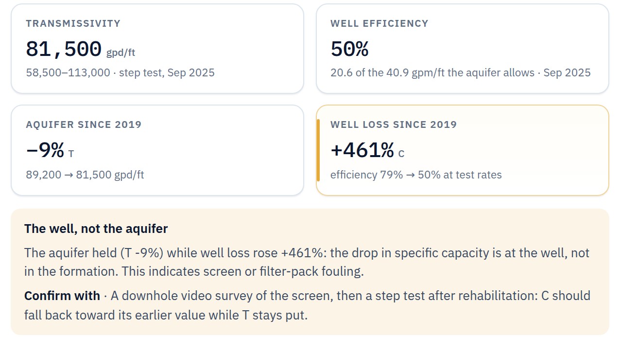
Case (a): the well. T and B have not moved; C has doubled, and well loss at 1,200 gpm went from 14.4 to 28.8 ft. Rising C with steady T is an indication of added loss at the screen, the gravel pack or the formation against it, such as encrustation, biofouling or fines. It is not yet a diagnosis: a downhole video survey shows what is there, and a step test after rehabilitation confirms what came back. If rehabilitation returned C to 1.0 × 10⁻⁵, drawdown would fall 14.4 ft and SC would return to 18.75 gpm/ft. For the wider question, see our note on a well producing less water: pump, screen or aquifer.
Case (b): the aquifer. C has not moved, but the slope steepened to 8.2 ft per log cycle: T = 264 × 1,200 ÷ 8.2 = 38,634 gpd/ft, 23.2% lower, and B rose with it. The static level fell 30 ft over the same years. Falling T with a falling static level is an indication that the aquifer delivers less per foot of drawdown, for example because the lower level has drained the top of a producing zone: where the head falls below the top of a confined zone, that zone turns unconfined and its saturated thickness shrinks, and T is conductivity times saturated thickness. Water levels in nearby wells confirm whether the decline is regional, and the screened intervals on the well log, set against the new static and pumping levels, show whether producing zones have drained. A camera will not find this, and rehabilitation will not bring it back. The pumping level at 1,200 gpm is now 288.1 ft, 44.1 ft deeper than at year 0; check it against the pump setting.
Run the specific-capacity rule on year 5 and it gives about 30,600 gpd/ft for case (a) and 30,700 for case (b). The rule cannot tell the two apart. Transmissivity and C can.
What makes a transmissivity trend worth trusting?
A trend compares tests, so the tests have to be comparable. Record each time:
- The method, kept the same: Cooper–Jacob against Cooper–Jacob, recovery against recovery. A method’s bias largely cancels when it is compared with itself.
- The pumping rate as measured at the well, and a similar test length.
- The minutes the line was fitted through, after casing storage and before any boundary or leakage bend.
- The static level after the well has rested, and the pump setting depth.
- A step test alongside, so C is tracked with T.
Every tested well in Waterwell IQ carries a transmissivity from the strongest test on file — constant-rate (Cooper–Jacob), recovery (Theis recovery) or a step test’s aquifer loss — with the method and the range it is sure within, tracked over time. Specific capacity alone is shown as a lower bound; the Waterwell IQ methodology page has the details.
Quick answers
Can you get storativity from the pumping well?
Not reliably. At the pumping well the line’s position depends on well loss and on an effective radius nobody measures, so S computed from it carries both errors. The USGS treatment cautions that a pumped well’s effective radius is often hard to determine (Ferris and others, 1962). Storativity needs an observation well at a known distance.
Is 2,000 × specific capacity good enough for the well file?
As a first look, yes; as the record, no. It is an order-of-magnitude estimate built on assumed storativity, radius and time, and well loss pulls it down by the well’s efficiency. In the example it read 37,500 gpd/ft against 50,286 from the constant-rate test.
Does falling specific capacity mean the well needs rehabilitation?
Not by itself. Falling specific capacity with steady T and rising C points to the well, where rehabilitation can help. Falling specific capacity with falling T and a falling static level points to the aquifer, where it cannot. Read the constant-rate slope and run a step test before choosing.
See transmissivity read from the tests on your own wells. Request a walkthrough →
Sources
- Theis, C.V. The relation between the lowering of the piezometric surface and the rate and duration of discharge of a well using ground-water storage. Transactions, American Geophysical Union 16(2): 519–524. 1935. The nonequilibrium equation and the recovery method: residual drawdown as continued pumping plus an equal recharge well from the moment of shutdown.
- Cooper, H.H., Jr., and C.E. Jacob. A generalized graphical method for evaluating formation constants and summarizing well-field history. Transactions, American Geophysical Union 27(4): 526–534. 1946. The straight-line (Cooper–Jacob) method.
- Jacob, C.E. Drawdown test to determine effective radius of artesian well. Transactions of the American Society of Civil Engineers 112: 1047–1070. 1947. The step-test split of drawdown into aquifer loss and well loss, s = BQ + CQ².
- Ferris, J.G., D.B. Knowles, R.H. Brown and R.W. Stallman. Theory of aquifer tests. U.S. Geological Survey Water-Supply Paper 1536-E. 1962. T = 264 Q log(t2 ÷ t1) ÷ (s2 − s1) in gpd/ft and gpm; u generally less than 0.01 for the straight line; the 0.3 Tt ÷ r²S form; the Theis recovery formula; the caution on a pumped well’s effective radius.
- Driscoll, F.G. Groundwater and Wells, 2nd ed. Johnson Division, St. Paul, Minnesota. 1986. The specific-capacity rule, T ≈ 2,000 × SC (confined) or 1,500 × SC (unconfined), in gpd/ft.
- Halford, K.J., W.D. Weight and R.P. Schreiber. Interpretation of transmissivity estimates from single-well pumping aquifer tests. Ground Water 44(3): 467–471. 2006. How single-well Cooper–Jacob estimates hold up in confined and unconfined aquifers.